
A E Banner
Introduction
Global warming is the increase in the average global temperature of the Earth’s atmosphere, measured at a height of 2 metres above Earth’s surface, since the 1850 to 1900 period.
The mainstream GHG theory for global warming has always been based on the recognized ability of carbon dioxide and other “greenhouse gases” to absorb electromagnetic infrared energy of certain wavelengths, radiated from the surface of the Earth. But, it has a major problem in that it cannot take account of the primary energy emitted into the atmosphere by human activities, particularly since about 1980, and it cannot be modified to include this effect.
On the other hand, the Primary Energy theory proposed here provides a very simple, straight- forward method of explaining the temperature increase anomalies from 1980 to 2022.
Moreover, it can also include the effects of greenhouse gases, although in a very different way from the 30 years old theory.
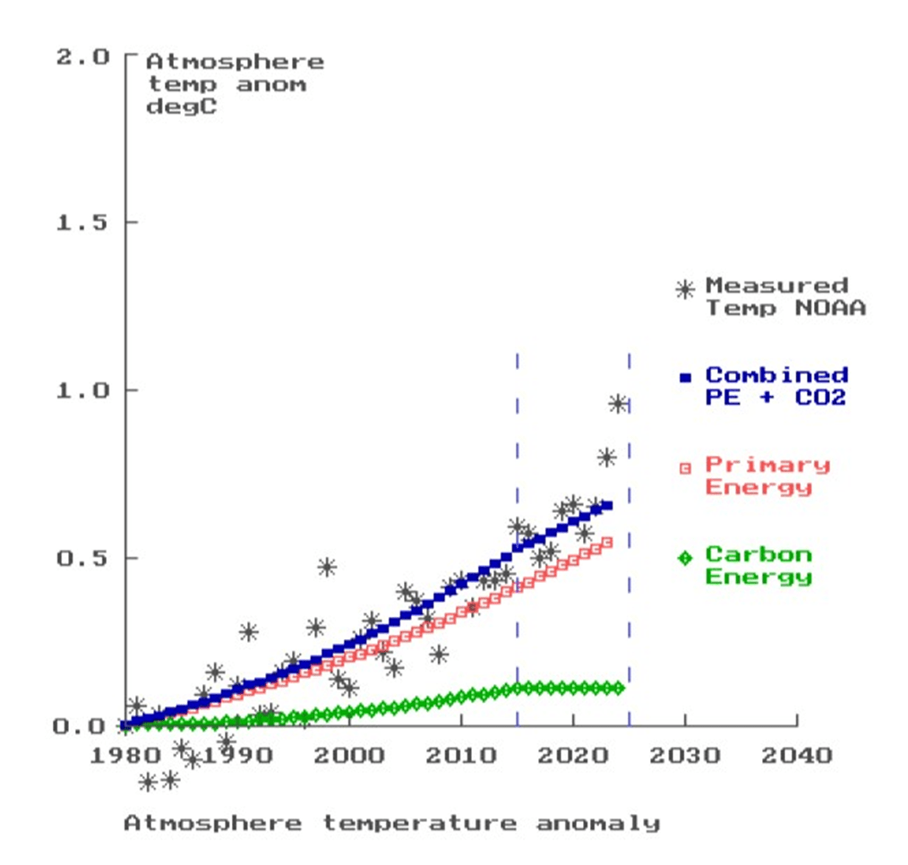
The temperature anomaly data has been obtained from NOAA (1), and is shown as “stars” in the graph below.
Primary Energy
Primary energy is the energy obtained from the internal energy of suitable sources such as fossil fuels. The chemical energy within the fuel is converted into primary energy when the fuel is burnt; for instance, in electricity power stations, automobiles, industry and agriculture.
Primary energy is emitted in the simple form of the kinetic energy of the extra hot molecules from the burning process. This is then shared among the atmosphere molecules by inter-molecular collisions, so raising the temperature of the atmosphere. Global warming!
The relationship between the increase in energy and resulting increase in temperature per air molecule is given by the Kinetic Theory as dE = (5k.dT) / 2 for diatomic molecules, where
k is Boltzmann’s Constant 1.381 * 10^(-23)
dE is the change in energy in Joules
dT is the change in temperature, in degrees C.
Data for the annual global amount of primary energy consumption have been obtained from “Our World in Data” (2), which itself is based on the BP Statistical Review of Energy. The annual data is in TWh for the whole Earth, which have then been converted for this work into average annual global Joules per square metre, J/m2, by considering the surface area of the Earth. So, the problem can then be considered by means of the “standard atmosphere column”, which is the column of the atmosphere, from the surface to the ToA, based on 1 m2 of the surface.
Much of the energy is used for various purposes, electricity generation, automobiles, industry and agriculture, but after use it reverts into simple “sensible” energy, ie kinetic energy. Any unused energy is in the same form, and so it also enters the atmosphere, and temperature is raised in line with the equation above.
It is important to realize that this extra energy in the atmosphere is in the form of the kinetic energy of the air molecules; it is not electromagnetic energy and so CANNOT be radiated away to space. However, some can return to the Earth’s surface, leaving some in the atmosphere, forming an energy aggregate which builds up year by year, so causing the atmosphere temperature to increase accordingly with the equation above. The proportion of the energy which is retained in the atmosphere, the “atmosphere energy retention factor”, is calculated in the Appendix.
The curve for primary energy is shown in the graph in light red squares. The temperatures are not quite sufficient to place the curve satisfactorily through the measured NOAA temperatures, but the “missing” energy is made up by the contribution from absorption by carbon dioxide, shown in green “diamonds”, so giving the curve for “Combined Energy” in blue squares. This contribution was determined by a “matching” factor applied to the CO2 curve.
Carbon dioxide in the atmosphere
Numerous internet sites show that the atmospheric concentration of carbon dioxide has been increasing substantially in a linear manner with time throughout recent decades. It has long been accepted that carbon dioxide in the atmosphere has the ability to absorb photons of electromagnetic energy at certain wavelengths in the infrared, radiated from the Earth’s surface; the amount of absorption being proportional to the atmospheric concentration of the carbon dioxide.
The initial ideas of the GHG global warming theory dating back more than 30 years have held that this absorption of energy reduced the output radiated out to space, and so upset the Earth’s energy balance condition. This required the surface temperature to rise in line with the Stefan-Boltzmann law in order that the radiation should increase, and so restore the energy balance.
While this theory has been the mainstream GHG theory since the late 1980s, it nevertheless has a fundamental problem which it is incapable of addressing. It completely ignores the major contribution of the Primary Energy, which is based upon energy being retained in the atmosphere.
The new Primary Energy theory proposed in this paper also includes the energy absorption properties of the so-called “greenhouse gases”, but offers a much simpler way of treating the outcome which does not depend upon radiation.
Absorption of energy by carbon dioxide
Fig 1 represents the annual energy absorption by atmospheric carbon dioxide of radiation from the Earth’s surface.
The CO2 concentration is increasing linearly with time, and so the absorption also increases correspondingly by the same amount each year. This extra annual addition of absorbed energy, for want of a better term, is called the “absunit”. It is not a fundamental constant, but refers only to the particular circumstances.
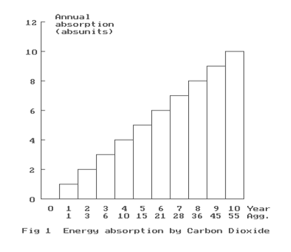
Starting with zero concentration in 1980, year number n=0, the energy absorbed is also zero.
So, in 1981, Year 1, n=1, the increase in absorbed energy is 1 absunit,
and so the absorbed energy is 1 absunit, and so the total absorption is 1 absunit.
In Year 2, n=2, the increase is 1, and so the total absorption is 2 absunits.
But, this is added to the total from Year 1, so the aggregate = 3 absunits.
In Year 3, n=3, the increase is 1, and so the total absorption is 3 absunits.
But , this is added to the total for Year 2, so the aggregate = 6 absunits.
Fig 2 provides the aggregates of retained, absorbed atmosphere energy
in absunits for 47 years.

Recent work by W Van Wijngaarden and William Happer, (3), shows that at a CO2 concentration of 400ppm, which was reached in 2015, virtually all of the radiated infrared energy at the relevant wavelengths was absorbed. Therefore, no extra energy can be absorbed by carbon dioxide even if further such gas emissions occur. This work is supported by Schack, (4) and Schildknecht, (5).
So, in 2015, n=35, the energy absorbed by CO2, and retained in the atmosphere is 630 absunits in Joules/m2, and when added to the primary energy it must raise the combined energy curve to provide a good fit to the NOAA measured temperature anomalies. The overall shape of the carbon curve is obtained from the table Fig 2.
It is then possible to calculate the values of the absunit in this application, and hence the atmosphere energy retention factor, as in the Appendix.
So, energy is absorbed by carbon dioxide molecules, causing a shortfall in the output to space. The mainstream GHG theory has always held that this shortfall must be made good by an increase in surface temperature in order to obtain greater radiation from the surface.
But, there is no data for any relevant increase in the global surface temperature.
However, the new proposed Primary Energy Theory does not require any such increase in surface temperature. Instead, it must explain the long-term measured increase in the temperature of the atmosphere. This is easily explained by the process called “thermalization”. The energy absorbed by the CO2 molecules increases the internal rotational and vibrational molecular energy, and this is transferred by collisions with “air” molecules, and so increases their kinetic energy and temperature.
The thermalization process is far more probable than radiation of a photon, and so takes preference. Prof W Happer has stated it is about a billion times greater. Ref (8).
Results
The graph shows the temperature anomaly curve in blue squares for the combination of the primary energy and the energy absorbed and re-emitted by carbon dioxide. This is referred to 1980, for which the published data gives the anomaly then as 0.27 degC with respect to the pre-industrial era.
The graph shows that the anomaly at 2023 is 0.65 degC with respect to 1980, and so the figure wrt the pre-industrial period is 0.92 degC.
This has not dealt with measured anomalies for 2023 and 2024 which are something of an enigma, and more data is required. But, perhaps another GHG is becoming apparent?
Conclusion
It is clear that up until 2022 the main driver of global warming has been the emission of primary energy from its source into the atmosphere, principally by the burning of fossil fuels in electricity generating power stations, in automobiles and transport generally, heating of buildings, and in industrial and agricultural processes. The effect of carbon dioxide is minimal.
So, any attempt to remove carbon dioxide from the atmosphere would be virtually useless. Probably worse, because any mechanism would be likely to involve the use of energy, so defeating its intention.
Before anthropogenic activities, the Earth’s system had achieved a stable temperature with the incoming energy from the Sun being balanced by the energy radiated away to space. The balance has now been disturbed by the primary energy emitted into the atmosphere by the burning of fossil fuels, energy which cannot escape.
Nuclear power, both fission and fusion, are unacceptable for the same reason; they put more energy into the atmosphere, and cause more warming.
Moreover, any other system which puts energy into the atmosphere must also be avoided. For instance, ground-source heat pumps, which simply move energy from below ground and then put it into the atmosphere. ( But, air-source heat pumps are excellent ).
Energy from the Sun is the most likely way to provide the required power for world consumption; both by solar panels and wind turbines. But, any attempt to obtain even more energy, like huge mirrors out in space, reflecting energy to receivers on Earth, are completely and totally unacceptable.
Appendix
To determine the atmosphere energy retention factor, a, and absunit, u
Consider the energy aggregates from 1980 onwards to any specified date.
Let P be the increase in aggregate Primary Energy emitted into the atmosphere, from 1980.
Let C be the increase in aggregate energy absorbed by carbon dioxide into the atmosphere, from 1980.
Some of the atmosphere energy is retained, but the excess flows to the surface.
Let a be the proportion retained in the atmosphere, ie the atmosphere energy retention factor.
Let R be the increase in total aggregate energy retained in the atmosphere, from 1980,
which includes both primary energy and the energy absorbed by carbon dioxide.
In each case, let the subscripts 0 and 5 denote the years 2000 and 2015 respectively.
( Ex. P5 is the aggregate primary energy for 2015 ).
Primary Energy Aggregate
The primary energy emitted annually into the global atmosphere from 1980 to 2023 were obtained in TWh from ( ), and then converted here into annual Joules per square meter of Earth’s surface. This annual data was then summed to provide the primary energy aggregate
which had entered the standard column from surface to ToA, based on 1 m2 of the surface.
So, P5 = 3.099 * 10^7 Joules/m2
and P0 = 1.549 * 10^7 J/m2
Combined Energy Aggregate (Pr.En + CO2 absorbed energy)
The Kinetic Theory of Gases states that for one molecule of a gas such as nitrogen or oxygen, which has two atoms per molecule, the change of temperature ΔT is related to the increase in energy aggregate ΔE by the following equation.
ΔE = (5/2) * k * ΔT where k = Boltzmann’s Constant, 1.381 * 10^(-23)
So, for the standard column with 2.04*10^29 molecules, the equation becomes
ΔE = (5/2) * k * ΔT * 2.04 * 10^29 J/m2
From the graph for the combined energy curve in blue, at 2015, ΔT5 = 0.530 degC,
and at 2000 ΔT0 = 0.247 degC,
The combined energy aggregates R5 and R0 retained in the atmosphere were then determined by means of the equation, as follows.
R5 = 3.7328 * 10^6 J/m2
R0 = 1.7361 * 10^6 J/m2
The combined energy aggregate R comprises the Primary Energy from fossil fuels and nuclear power and so on, plus the energy absorbed by carbon dioxide from the radiation from the Earth’s surface.
This total energy is emitted into the atmosphere, but only a small proportion is retained.
Let a = the atmosphere energy retention factor. This must be determined.
Therefore, in 2015 a(P5 + C5) = R5 ……………………..(1)
and in 2000 a(P0 + C0) = R0 ……………………..(2)
Divide (1) by (2) (P5 + C5) / (P0 + C0) = R5/R0 …………………………(3)
The aggregate values of the Primary Energies P5 and P0 which entered the standard column of the atmosphere are given above.
It is required to find the values for the carbon dioxide energies C5 and C0 .
The aggregate atmosphere energies C5 and C0 are shown in the table, Fig 2, in terms
of the “absunit”, for this set of primary and absorbed energy conditions.
Let u = the value of 1 absunit in Joules/m2
From the table, at 2015 where n = 35 there are 630 absunits, so C5 = 630u
and at 2000 where n = 20 there are 210 absunits, so C0 = 210u
Substitute these values in (3)
(P5 + 630u) / (P0 + 210u) = R5 / R0 ………….(4)
With a little algebra, we find the value of the absunit u for this calculation, including Primary Energy
u = (P0 .R5 – P5 .R0) / (630.R0 – 210.R5)
u = 1.297 * 104 Joules/m2 ……………………(5)
From (1) a(P5 + C5) = R5 and C5 = 630u
Hence, we find a = 0.0953
The atmosphere energy retention factor is 0.0953, or 9.5 %
Therefore, the energy returning to the surface is 90.5 %
These values are supported by NOAA (6) and IPCC (7).
References
(1) https://www.ncdc.noaa.gov/cag/global/time-series/globe/land_ocean/ann/
Select: Timescale Annual; Start Year 1970; End Year 2022; Surface Land and Ocean
(2) https://ourworldindata.org/energy-production-consumption
(3) Van Wijngaarden and Happer, https://arxiv.org/abs/2006.03098
(4) Schack, Phys.Blatter, 28 26 (1972)
(5) Schildknecht, https://arxiv.org/abs/2004.00708v2
(6) https://www.climate.gov/news-features/understanding-climate/climate-change-ocean-heat-content
(7) https://www.ipcc.ch/report/ar6/wg1/downloads/report/IPCC_AR6_WGI_Chapter07.pdf
(8) http://www.sealevel.info/Happer_UNC_2014-09-08/Another_question.html
(Go to Prof Happer’s response in upper case on Thurs, Nov 13, 2014 at 11.29 AM )
